

Part 1: Matching accuracy metrics for patient tokenization in healthcare
[Part 1] of Matching Accuracy Metrics
Catch up on Part 2, Part 3 and Part 4
By: Austin Eliazar Ph.D., Chief Data Scientist, HealthVerity
As the volume of digital patient data grows, so does the need for accurate patient tokenization in healthcare. Privacy-preserving record linkage (PPRL) offers a privacy-safe solution, but how do you measure its accuracy? Meeting this need for extensive longitudinal linking in a way that preserves people’s privacy has become critical, and there are more and more companies who claim to solve that problem for you.
Read the full Matching Accuracy Metrics White Paper
However, not all solutions are equally effective. Missed links (false negatives) leave your data fragmented and useless. Incorrect links (false positives) add errors to the individuals’ profiles and can lead your analysts to the wrong conclusions. It can be difficult to cut through the hype and understand how accurate a system truly is in real-world conditions, especially when all of the data has been de-identified. Fortunately, there are plenty of ways to objectively evaluate the performance of an anonymized system in an anonymized way, so that we can tell if a solution is too good to be true.
In this 4-part series, we will focus on quantitative evaluations and how to compute them on an anonymized data set. Our focus will be on practical methods with intuitive behavior. In the first part, we focus on simulation and surrogate methods which use real data with approximate ground truth. Next, we will focus on indirect methods for big data, with separate parts devoted to false positives and false negatives. We conclude with a series of soft indicators that provide bounds on the accuracy for common pain points in data linkage.
Defining matching accuracy metrics for healthcare data linkage
To evaluate the performance of a matching system, we need hard, quantitative numbers that capture how well the system is really doing. There are two key types of failures that we are concerned with: False positives and false negatives. False positives are errors where two or more individuals are treated as the same person. Essentially, the matching is too aggressive and, because of that, makes additional links that don’t actually exist. This type of error can be costly to analytics, as it adds false correlations and increases the noise. This can lead to erroneous or even contradictory conclusions. If you can’t keep your individuals separate and distinct, all of the benefits of longitudinal linking are lost. False negatives are errors where a single individual is represented as more than one person in the data. In effect, the matching is being too conservative or missing cues, resulting in a fragmented view of an individual. This type of error costs more than just a missed opportunity and can lead to duplicative efforts, overestimates of cohort populations, or blind spots to key indicators. It isn’t always clear where the link was missed and what data is now missing. If the links cannot be made reliably, you may be better off not linking at all.
Clearly, these errors represent opposing efforts — if you are very aggressive, you can always achieve zero false negatives, but the number of false positives is likely to be prohibitively high. On the other hand, you can trivially achieve zero false positives by just not even trying to link the data, but your false negatives are through the roof. A good system will be able to keep both types of errors low at the same time, while still allowing some flexibility in the tradeoff. However, that tradeoff isn’t always consistent, and it is important to find a system that performs well at the right tradeoff point for you.
In this series, we quantify these two key factors in the simplest terms of false positive rate (FPR) and false negative rate (FNR). Numerically, that means FPR = (number of false positives) / (population size) and FNR = (number of false negatives) / (population size).

In different literature you may see other terms, such as sensitivity and specificity, or precision and recall. These are all different ways of representing the same tradeoff, and can easily be derived from the FPR and FNR.
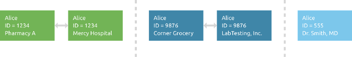
Here we are defining a false positive as anytime an additional person gets assigned to the same ID in the system. So if ID=1234 is associated to a prescription from Alice, a diagnosis from Bob, and a credit card purchase from Charlie, that counts as two false positives — one for each person after the first. Similarly, a false negative is anytime an additional ID gets assigned to the same person. So if Alice’s prescriptions are listed under ID=1234, but her ER visit is under ID=2345, and her grocery data with the vitamin supplements is under ID=3456, then that counts as two false negatives — two missed chances to link disparate data. As you can see, the FPR and FNR can even go higher than one. If the three IDs above each have some data from each of the three people in the population, that’s six false positives (two additional associations from each ID) and six false negatives (two additional fragments from each person), giving a FPR and FNR of 6/3=2.
Keep in mind when testing the accuracy that attempting to link more data sources or sites will likely increase both types of error. All of the records from a single pharmacy location will likely have the same information for a single person, making it straightforward to maintain a single ID per person. Adding a payer to the system provides a limited number of opportunities for both false positives and false negatives for each person. However, adding multiple payers, along with multiple pharmacies and multiple doctors will increase the number of both type of errors, even if the system is performing just as well for each new chance to link. For this reason, it is important to take context into account when comparing error rates.
Evaluating healthcare tokenization accuracy with privacy- preserving-record linkage (PPRL) metrics
Testing the matching accuracy of an anonymized system is very difficult. The nature of the data means that ground truth is rarely available, and the very factors that aid in linking are obfuscated or removed, making human review impossible. For this section, we focus on surrogate systems, where measuring the accuracy is the most obvious and intuitive. However, these tests are filled with hidden pitfalls, making them often the least reliable and least informative tests. So the tests in this section are a good first pass to understand the matching behavior, while the additional tests we describe later in this series are critical to verify the performance.
Testing healthcare data linkage: Simulation methods
One of the most obvious ways to test a system is to create a synthetic data set to test on.
Start from real data. To make the simulations as representative as possible, it is best to simulate as little as possible. Starting from a real data set will help capture natural distributions in names and demographics, as well as any hidden correlations. If the data is missing key fields for matching, draw from representative sample distributions wherever possible, such as US Census data.
Push the boundaries. Every matching system has certain assumptions built in. It is important to know how the system behaves when those assumptions are put to the test. While gross violations are not very useful (e.g. swapping in a doctor’s name for the patient name is just going to make most systems fail) and extreme variations are not plausible (e.g. everyone changing addresses every month), pushing the system to have three times more or less typos can test how the system will perform on data that varies over time or across different data partners.
Keep an open system. The temptation in any simulation is to assume that everything is known ahead of time. Typically, simulations are built where set A and set B cover the same population of people, and any referential databases or distributions are complete and up to date. However, it is important to keep in mind that any group of people will be constantly adding and losing individuals, and the underlying distributions can change dramatically in just one year. Allowing an open system — where people can come and go — in your simulations will test important aspects of the matching system that are needed in real world scenarios.
Keep an open mind. Always remember that simulations are not the real world and are limited by humans who made them. This can work in both directions, too. A simulation and a matching system built by the same people are likely to have the same assumptions, consciously or not, and can easily perform much better because of this. However, simulations are often oversimplifications of real world data, and they fail to include patterns and structure in the data that a good learning system can take advantage of. These differences can be especially apparent when two matching systems are tested on the same simulation. So, while a simulation can provide clean quantitative measures, it’s not always clear if those measures are better or worse than how the system handles data in the wild.
Using surrogate identifiers to validate PPRL accuracy
Perhaps the truest method of testing a matching system is to use a data set with surrogate identifiers to use as a ground truth. A reliable ground truth, such as a Social Security Number (SSN) can be hashed and withheld as a ‘gold standard’ to match against. However, these are very difficult to obtain, especially across multiple data sets. Any data with reliable ground truth will likely be much smaller and much better behaved than the type of data sets you want to test for. Also, many of the surrogate IDs that you may be tempted to use are themselves flawed. Human labelled sets are laborious and deeply biased. Plaintext matching systems are often not much better than anonymized matching and can suffer from many of the same types of weaknesses. Maiden names, twins, nicknames and cross-country moves are just as likely to trip up human or a “gold standard” matching system, and do not give a decent measure of either FPR or FNR. If the surrogate identifier is not as accurate and complete as a Social Security Number, it is best to not use it.
If you are lucky enough to have a large system with a ground truth attached, that is one of the best measures to use. However, here are a few caveats to keep in mind with these tests:
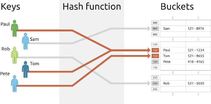
Hash collisions. Hash collisions are a common occurrence where unique identifiers are ‘randomly’ mapped to a new set of values, but bad luck and the birthday problem mean that different starting values can be mapped to the same hashed value. It’s important to quantify the expected frequency of these collision rates for your ground truth identifier and subtract that from your FPR accordingly. The collision rate can be calculated mathematically or through simulation. Each collision will look like a false positive, when in fact it is not, and the expected number of collisions can be subtracted from the observed number of false positives before computing FPR. If the collision rate is high or the original identifier space was not necessarily unique (e.g. using the last four digits of SSN), it may be helpful to quantify how often you are accidentally correct and add that to the FNR. This is because sometimes the matching system can miss a link between two IDs, but coincidentally, those IDs happen to map to the same value in the hash space. In adjusting the FNR, keep in mind:
(observed false negatives) = (true false negatives) * (1 — collision rate).
Typos in the ground truth identifiers. Matching is difficult because the data is dirty. Typos and transcription errors occur regularly in all fields and the ground truth identifier is not immune. An identifier with some built-in error detection (such as a checksum or parity bit) is always preferred, but rarely used. A best effort should be made by someone with access to the plaintext data to quantify the typo rate. If that is not available, a distance preserving hash of the identifier could be useful for someone with the anonymized data to put upper and lower bounds on the likely typo rate. The typo rate can then be used to adjust the observed number of false negatives.
Sample context. The results of any tests using surrogate identifiers should be taken with a grain of salt. While the metric numbers are likely very accurate, the context of the data is not going to be representative of real-world challenges. Test data with a reliable ground truth is going to be more complete, more homogenous, less noisy, and better behaved than you will see in other situations. In that sense, the results should be treated much like the simulated matching tests — a theoretic estimate of accuracy when everything is generally obeying the expectations and assumptions that are built into the matching system. This is a valuable measurement, but it still needs to be validated by other means to test the robustness in the wild.
To ensure your healthcare tokenization solution meets PPRL standards, benchmark your false positive and false negative rates using real-world data and surrogate testing methods outlined here.
Continue reading Part 2, Part 3 and Part 4
Interested in learning more about matching accuracy?
Get the full white paper here.


