

Part 3: Measuring false negatives in anonymized healthcare data
[Part 3] of Matching Accuracy Metrics |
Catch up on Part 1 and Part 2, or read Part 4
By: Austin Eliazar, Chief Data Scientist, HealthVerity
False negatives, the missed links between records, are the most obvious errors in a matching system. They can be easily seen in low match rates, short histories, and isolated records. However, it can be difficult to tease apart how many of these problems are coming from missed matches and how many are from honest gaps in the data coverage. In this section, we focus on the challenges introduced by false negatives and present solid ways to measure the false negatives without resorting to artificial scenarios like simulation or well-controlled ground truth.
Read the full Matching Accuracy Metrics White Paper
What false negatives are and why they matter
False negatives in matching represent a job half done. Correlations between data sets are weak and only partially complete, leaving the data fragmented and isolated. This problem is compounded by each new data source, as each additional source provides a new set of broken links, leaving the data fragmented and siloed all over again. False negatives dilute the effectiveness of your data, negatively affecting your analysis in several ways:
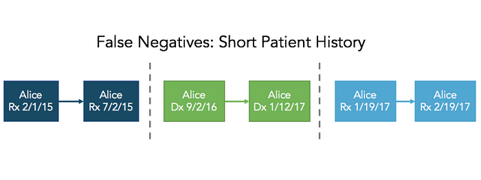
Short patient history: Whether the false negatives happen across providers or within a single system, they can severely limit the duration of a patient history. Twenty years of historical data can be rendered moot if the false negative rate (FNR) is limiting the average patient history to three years. Short histories can significantly limit the effectiveness of the analysis, especially when looking for cause and effect, long term side effects and outcomes, or survivability.
Narrow patient history: False negatives affect the width of the patient history even more significantly, making it difficult to get a full picture of the patient activity. Most analysis these days focus on the whole patient journey, with insights into medical, pharmacy, and lab data as a minimum set, with additional behavioral and purchase histories commonly being added. Adding more complexity, most patients will have history at multiple lab or pharmacy sites, further expanding the breadth of linking necessary. High FNR limits the number of additional data types that can be associated with the patient journey, giving a narrow, myopic view of the patients, leaving most of your valuable data behind.

Failed indexes: Weak linking affects the discovery process just as much as histories. Using a matching system for the initial discovery phase means FNR has a major impact on discovering re-enrollment, prior conditions, or data purchasing. In many of these cases a false negative is not just diluting the results, but it is providing false conclusions. This can have as much danger in skewing the results as a false positive, as the presence or absence of an event can be just as important as the result.

Using match rates to estimate false negatives
One approach to measuring the FNR is to look to match rates, leveraging the failed indexes as a measure of false negatives. By looking at the first time a new data source is matched against an existing base dataset, we can use the cold start match rate as an approximation of the false negatives. This provides an easy, obvious measurement, but is often noisy and easily biased. Extreme care must be taken to control for common sources of inaccuracy.
This measurement is computed using an existing base dataset — comprised of one or many different data sources — and a new incoming data source, which has never been included in the base dataset before. The incoming dataset is matched against the base dataset, then the number of shared identities between the two data sets is counted. Any records in the incoming data that don’t match to the base set are matched against each other to deduplicate these new identities. We calculate the total negative rate as
Total negative rate = (number of shared IDs) / (total number of incoming IDs)
Keep in mind that this rate includes both false negatives and true negatives. The key to this method is to reduce and remove as many sources of true negatives as possible, until all that is left is the FNR. Here are a few pointers to help with that:
Regional coverage. This measurement method only works well if there is good overlap between the data sets. Otherwise, the false negatives and the true negatives are intermingled. You can boost the overlap if you only use identifiable subsets — such as specific zip codes and/or age brackets — where the base data set has high coverage. Creating these subsets and comparing the identity counts against known census figures can help in finding sections with sufficiently high coverage.
Baseline noise. Certain amounts of noise are going to be present, even in a perfect matching system. Input data is not perfect and may have invalid records or dummy values included. Also, the population itself is in flux, with people moving in and out, plus new births and deaths. To get a good estimate, you need to subtract this baseline from the observed negatives. The baseline noise can be computed from outside sources, but it requires good external statistics combined with an accurate sense of the average update rate of individual records. Depending on your data sources, you could also estimate this from the incoming data feed itself, by matching the data set against itself. Although this baseline estimate will also be affected by false negative and false positives, data sources with a high record frequency and good internal consistency will have far fewer errors than matching across data sources.
Repeated tests. Each data source has its own eccentricities that can cause stark differences in initial matching. Issues of coverage, noisy input, invalid data, and dummy data can cause wide variation. That is why it is critical that this test is repeated over many different sources. The goal is to get an average sense of the FNR across all types of data sources. Using three different sources is a bare minimum to be aware of outliers, while eight or more are good to get a reliable estimate.
A probabilistic approach to measuring missed matches
In any random set of people, there is a chance that some pair of them will share the same birthday. This is not surprising since there are only 366 possible birthdays (including February 29). What may be surprising to you is how often this happens in small groups. In a group of 100 people, on average 24 of them will share a birthday with someone else. Even in a group as small as 23, there is a >50% chance that there will be at least one shared birthday. For just about every identifier in a matching system, from age to zip code, these duplications happen regularly and at a reliable rate. That’s part of why identity matching is so hard.
Fortunately, we can use these random duplicates to measure the false negative rate. The basic reasoning is simple — missed links result in extra data. We know how often duplicates should occur, so we can check and see how close the duplicate rates are in our matched identities. The number of missing duplicates is a measure of false positives.
The key to making this idea effective as a metric lies in choosing small groups, where each group would have held the identities of both of the people in a false positive if they hadn’t been merged together. Choosing groups along some of the more reliable identifiers is effective. For our example, we will consider a group of matched individuals who all share the same tokenized name. Of course, there are plenty of name tokens to choose from, so we can choose one with a reasonable size, say 100 individuals. Within this group, we use birthdays as our test field, and count the number of duplicate birthdays. We compare the observed number to the expected number of duplicates — in this case 24 — and figure out the difference. In some instances we will see more or less, just based on sampling errors. However, if we take the average over a large number of similarly sized groups, the noise dies down and any overcount is a sure sign of false negatives.
It is important to keep in mind that the number of duplicates is affected by false positives as well as false negatives. Incorrect data links often are triggered by these coincidental matches. These false positives then drive down the number of observed duplicates. When using this method to measure FNR, it is important to have a reliable estimate of FPR from an independent test (such as the post mortem activity, as described in our previous blog).
FNR = (average observed duplicates) — (expected duplicates) + FPR
Duplicate rates: The rate of duplicates in a group depends on the size of the group, the range of the test values, and the natural distribution of those values. You can find the expected value for the number of duplicates using mathematical equations, but these often assume the values are uniformly distributed. If you have enough individuals in the matching system (which most matching systems do), you can measure the value distribution empirically from the data and simulate appropriately sized sample groups. The FNR is assumed to be low enough and largely independent of the test field so as to not significantly skew the results.
Sample errors: For testing, more is better. The number of groups that you use in your average affects the precision of this test, and using more groups is more reliable. Sample error calculators are very helpful to quantify your margin of error.
Selection bias: Keep in mind that the choice of fields to use — both for group selection and for duplicate measurement — can affect your results. Really, the example above is only measuring the number of false positives where the name and birthday matched. If the source data for one of these values is often noisy, you will miss any false negatives that are made outside of your selected group. Repeating this test across different pairs of fields can give different views of the FNR, and even give insights into where the system may be stronger or weaker.
Continue reading Part 4.
Interested in learning more about matching accuracy?

